from sklearn.model_selection import train_test_split
from sklearn.feature_selection import RFE
import pandas as pd
import numpy as np
data = pd.read_csv("biomechanics_dataset_v1.csv") 
np.random.seed(1)

X = data.iloc[:,1:60]
y = data.iloc[:, 60]
x_train, x_test, y_train, y_test = train_test_split(X,y, test_size = .2)
#Set up

from RandomForestRegressor import RandomForest

rf = RandomForest()

rf.fit(x_train, y_train, 1000, 500)

We also chose to implement and train a second model on our data. We implemented Random Forest Regression, since it is a very powerful model for making predictions with continous data. When we train this model on our whole data set, we get a much better validation score than with linear regression. However, just like with linear regression we can use feature reduction to reduce overfitting.

rf.score(x_test, y_test)

0.5699951488283441

from sklearn.ensemble import RandomForestRegressor
from sklearn.feature_selection import RFE
model = RandomForestRegressor()
scores = []

for x in range(60):
    estm = RFE(model, n_features_to_select = x+1, step = 1)
    estm.fit(x_train,y_train)
    scores.append(estm.score(x_test,y_test))

import matplotlib.pyplot as plt

x_val= [] 

for j in range (60):
    x_val.append(j+5)

  
plt.plot(x_val, scores)  # Plot the chart
plt.xlabel("Number of Features")
plt.ylabel("Validation Score")
plt.title("Random Forest Regression")
plt.show()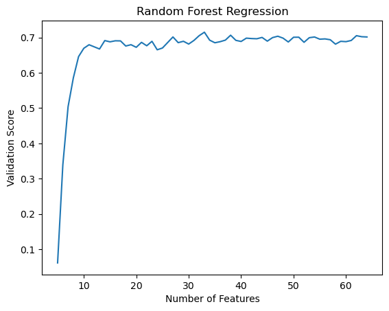 

We can see that this machine doesn’t suffer as much from overfitting, and has a higher validation score than Linear Regression.

x_train = x_train.iloc[:,[1,8,13,18,21,26,29, 34,38, 46,48,55,56,58]]
x_test = x_test.iloc[:,[1,8,13,18,21,26,29, 34,38, 46,48,55,56,58]]

rf.fit(x_train, y_train, 1000,500)
rf.score(x_test, y_test)

Using the features we found from our RFE we get this score.